Instrumentation & Process
Control Guide
Transfer functions, dynamic modeling, block diagrams, stability, and PID controller tuning for the GATE Chemical Engineering paper.
Overview
Instrumentation & Process Control is the section that asks not "what does this process do at steady state" but "how does it behave when something changes, and how do we keep it on target." In the GATE CH syllabus it draws on classical control theory (Laplace-domain transfer functions, block diagrams, stability criteria) applied specifically to chemical process dynamics, tanks, heat exchangers, and reactors modeled as first- or second-order systems.
The syllabus builds from dynamic modeling to control design. First, processes are modeled as transfer functions, first-order (a single tank or thermal system), second-order (interacting tanks, underdamped systems), or first-order-plus-dead-time (FOPDT), each with a characteristic step response shape. Next comes control-loop analysis: block diagram algebra to reduce a full feedback loop to a single closed-loop transfer function, then stability analysis (Routh-Hittaway/Routh array, root locus intuition) to check whether a proposed controller will keep the loop stable. Finally, controller design and tuning (P, PI, PID actions, Ziegler-Nichols tuning rules) and control-system architecture (cascade, feedforward, ratio control) round out the syllabus.
This section rewards fluency with Laplace transforms above almost anything else, nearly every numerical starts by converting a differential equation or a described physical system into a transfer function G(s), then manipulating it algebraically. The standard reference is Coughanowr & LeBlanc's "Process Systems Analysis and Control," whose derivation style (first-principles balance → linearize → Laplace transform → transfer function) mirrors exactly how GATE frames these problems.
Real GATE CH PYQ Frequency (2024–2026)
| 2024 | 2025 | 2026 | 3-Yr Avg |
|---|---|---|---|
| 5 | 5 | 5 | 5 |
Computed directly from 15 real questions tagged to this topic across our GATE CH 2024–2026 archive, averaging 5 questions/year. Browse the underlying 15 questions for this topic in the PYQ archive, or see the full topic weightage comparison across all topics.
GATE Weightage
Process Control typically contributes 4–6 questions (about 7–11 marks) to the GATE CH paper, spread across transfer function modeling, block diagram/stability analysis, and controller design/tuning.
| Sub-area | Approx. Marks |
|---|---|
| Transfer functions & dynamic modeling | ~2–3 |
| Block diagrams & closed-loop transfer functions | ~1–2 |
| Stability analysis | ~1–2 |
| Controller types, tuning & control architectures | ~2–3 |
Sub-area split is a directional estimate (our archive doesn't tag marks at this granularity), for the real, computed topic-level total, see "Real GATE CH PYQ Frequency" above.
Key Subtopics
First-order systems
The standard first-order transfer function K/(τs+1), its step response (63.2% of the way to final value at t = τ), and physical examples like a stirred tank with inlet composition changes.
Second-order systems
Underdamped, critically damped, and overdamped responses characterized by the damping ratio ζ and natural frequency ωn, overshoot and settling time both depend directly on ζ.
Dead time & FOPDT models
First-order-plus-dead-time models approximate higher-order or nonlinear process dynamics for controller tuning purposes, with the dead time θ representing pure transport delay.
Block diagram algebra
Reducing a feedback control loop (process, sensor, controller, final control element blocks) to a single closed-loop transfer function relating output to setpoint and disturbance.
Stability analysis
The Routh array (or root-locus reasoning) applied to the closed-loop characteristic equation to determine the range of controller gain that keeps the loop stable.
Controller types (P, PI, PID)
Proportional, integral, and derivative control actions, P offers offset but fast response, I eliminates offset but can destabilize, D adds damping but amplifies noise.
Controller tuning
Ziegler-Nichols (both open-loop reaction-curve and closed-loop ultimate-gain methods) as the standard rule-of-thumb approach to picking initial PID tuning parameters.
Advanced control architectures
Cascade control (an inner fast loop correcting disturbances before they propagate), feedforward control (measuring a disturbance directly), and ratio control for blending processes.
Essential Formulas
Full formula reference →Standard first-order transfer function; K = steady-state gain, τ = time constant
First-order step response to a step input of magnitude A
Standard second-order transfer function; ζ = damping ratio (ζ < 1 underdamped, oscillatory)
FOPDT (first-order-plus-dead-time) model; θ = dead time / transport delay
Standard closed-loop (setpoint-tracking) transfer function for a unity-feedback control loop
PID controller action in the time domain (Kc = controller gain, τI = integral time, τD = derivative time)
Steady-state offset, nonzero for proportional-only control under a sustained load change, zero once integral action is added
Ziegler-Nichols closed-loop (ultimate gain) PID tuning rule
Visual Reference
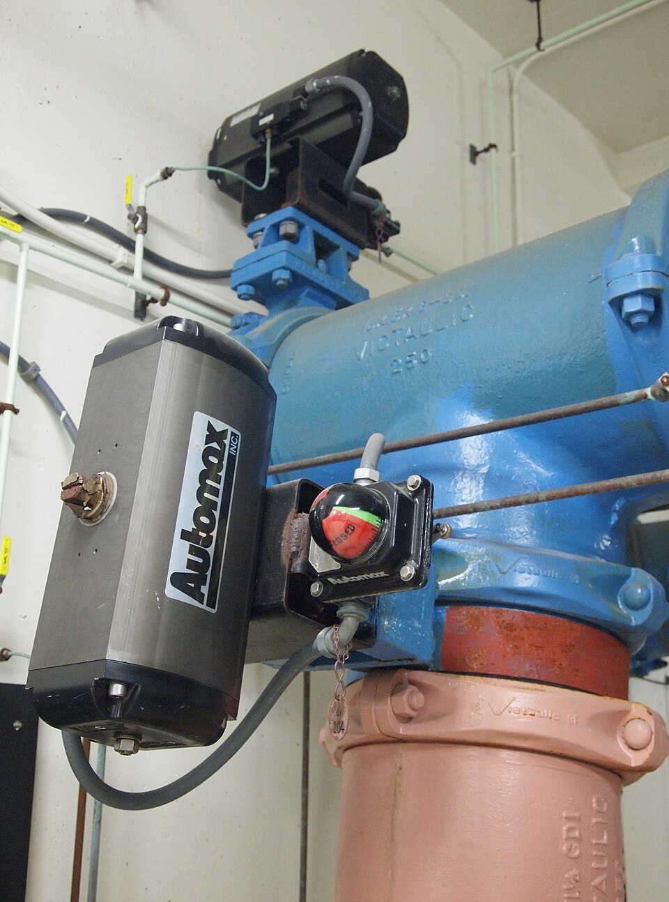
Derivations & Physical Insight
From a Stirred-Tank Energy Balance to a First-Order Transfer Function
Consider a well-mixed tank at temperature T, heated by an inlet stream at temperature Ti with flow rate F, volume V constant. An unsteady-state energy balance around the tank gives a first-order linear ODE in T. Deviation variables (T' = T − T_ss, Ti' = Ti − Ti,ss) remove the steady-state constants, and Laplace-transforming the resulting linear ODE (assuming zero initial deviation) converts differentiation into multiplication by s:
Why Integral Action Eliminates Offset (and Proportional-Only Control Cannot)
Under proportional-only control, the controller output is u = Kc·e, where e is the error between setpoint and measured value. At steady state after a sustained load (disturbance) change, the process needs some nonzero controller output to hold the new steady state, but a nonzero output under pure proportional control requires a nonzero error, by definition of u = Kc·e. That permanently nonzero error at steady state is exactly the offset, and no finite Kc can drive it to zero without also driving the required controller output to zero, which contradicts what's needed to counteract the disturbance.
Integral action breaks this constraint because it accumulates error over time rather than reacting only to its instantaneous value: u includes a term (1/τI)∫e dt, which keeps growing (or shrinking) as long as any error persists at all. The only way for that integral to stop changing, i.e., for the system to reach a new steady state, is for the error itself to reach exactly zero, since a nonzero constant error integrated over infinite time would diverge. This is the structural reason integral control always eliminates steady-state offset for a sustained (step-like) disturbance, at the cost of potentially slower or more oscillatory transient response.
Worked Practice Problems
Original practice problems in the GATE CH style, not copied from any question bank. Work them before reading the solution.
First-Order Step Response, Time to Reach 90% of Final Value
Problem: A first-order process (K = 2, τ = 5 min) is subjected to a step input of magnitude 3. Find the time required for the output to reach 90% of its final steady-state change.
Given: K = 2, τ = 5 min, step magnitude A = 3, target = 90% of final value.
Answer: t ≈ 11.5 min (independent of K and the step size, 90% response time is always 2.303τ for a first-order system).
Ultimate Gain and Period from a Marginally Stable Loop
Problem: A closed-loop system with proportional-only control becomes marginally stable (sustained oscillation) at a controller gain Kcu = 4, with an observed oscillation period Pu = 6 min. Using the Ziegler-Nichols closed-loop method, find the recommended PID settings (Kc, τI, τD).
Given: Kcu = 4, Pu = 6 min. Ziegler-Nichols PID rule: Kc = 0.6Kcu, τI = Pu/2, τD = Pu/8.
Answer: Kc = 2.4, τI = 3 min, τD = 0.75 min.
Topic-wise PYQ Frequency
Transfer functions & dynamic modeling
GATE 2025 Q25/Q39 (transfer functions) and GATE 2026 Q60 (FOPDT modeling) show this is tested almost every year.
Controller types & tuning
GATE 2024 Q64 (PD control), GATE 2026 Q44 (control valves) and Q50 (Ziegler-Nichols tuning) confirm regular testing.
Block diagrams & closed-loop analysis
GATE 2024 Q48 tested block diagrams directly, a recurring conceptual/numerical style.
Advanced architectures (cascade, feedforward)
GATE 2024 Q22 (feedforward) and GATE 2026 Q62 (cascade control) show these are tested periodically.
Sensors & instrumentation dynamics
GATE 2026 Q51 tested a first-order sensor model, instrumentation-specific questions appear less often than pure control-loop ones.
Level & distillation column control
GATE 2024 Q23 (distillation control) and Q63 (level control) show applied control-loop scenarios do appear, if less frequently than the underlying theory.
Recommended Study Order
- 1
1. Laplace transforms & first-order systems
The mathematical prerequisite for this entire section, get comfortable transforming ODEs before anything else.
- 2
2. Second-order & FOPDT systems
Extends first-order intuition to underdamped/dead-time behavior, both common in GATE numericals.
- 3
3. Block diagram algebra
Needed to reduce any described control loop to a single transfer function before analyzing stability or tuning.
- 4
4. Stability analysis (Routh array)
A direct, mechanical procedure once the closed-loop characteristic equation is known, high value for the effort required.
- 5
5. Controller types (P, PI, PID) & tuning
The highest-yield applied subtopic, practice both Ziegler-Nichols methods and offset reasoning for each controller type.
- 6
6. Advanced control architectures
Lower frequency, a conceptual pass on cascade, feedforward, and ratio control is usually sufficient.
Common Pitfalls
✗ Forgetting to convert to deviation variables before Laplace-transforming a process model.
✓ Steady-state terms don't transform cleanly, always subtract the steady-state value first so the ODE (and its transform) starts from zero.
✗ Assuming proportional-only control can eliminate offset with a large enough gain.
✓ No finite Kc eliminates offset under P-only control for a sustained disturbance, only integral action can, at the cost of potential oscillation or instability at high gain.
✗ Confusing the two Ziegler-Nichols methods (open-loop reaction curve vs. closed-loop ultimate gain) and mixing their formulas.
✓ The open-loop method uses a step-test reaction curve (process gain, time constant, dead time); the closed-loop method uses the ultimate gain Kcu and period Pu from a marginally stable loop, check which data the problem gives before picking a formula.
✗ Ignoring dead time when assessing closed-loop stability.
✓ Dead time adds negative phase lag that pure first/second-order transfer functions don't capture, a system that looks stable without accounting for θ can become unstable once dead time is included.
Put It Into Practice
Work through the step-response and Ziegler-Nichols problems above with Laplace-domain reasoning at each step, then apply the same transfer-function approach to the process control questions in the full GATE previous-year test set.
Keep Exploring
Related
Chemical Reaction Engineering
Rate laws, ideal reactors (batch, CSTR, PFR), RTD, non-ideal flow, and catalysis for GATE CH.
Open →Process Calculations
Material & energy balances, recycle/bypass/purge systems, and combustion stoichiometry for GATE CH.
Open →GATE CH Formula Sheet
Every core GATE Chemical Engineering formula in one place, grouped by topic with variable definitions.
Open →GATE Practice Tests by Year
Full-length, timed GATE CH practice tests (2024–2026) with instant, step-by-step-explained results.
Open →